Here is for each application a simple procedure to be sure that everything is well installed
Datxplore
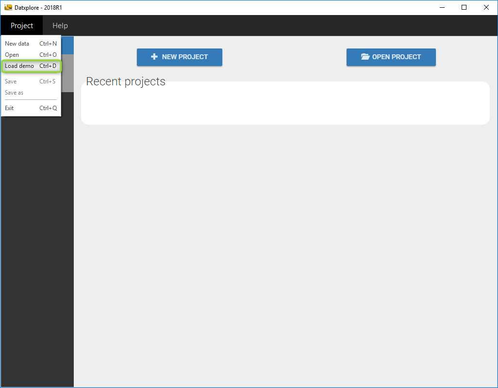
- Open Datxplore
- Go to the menu Project/Load demo as on the following figure
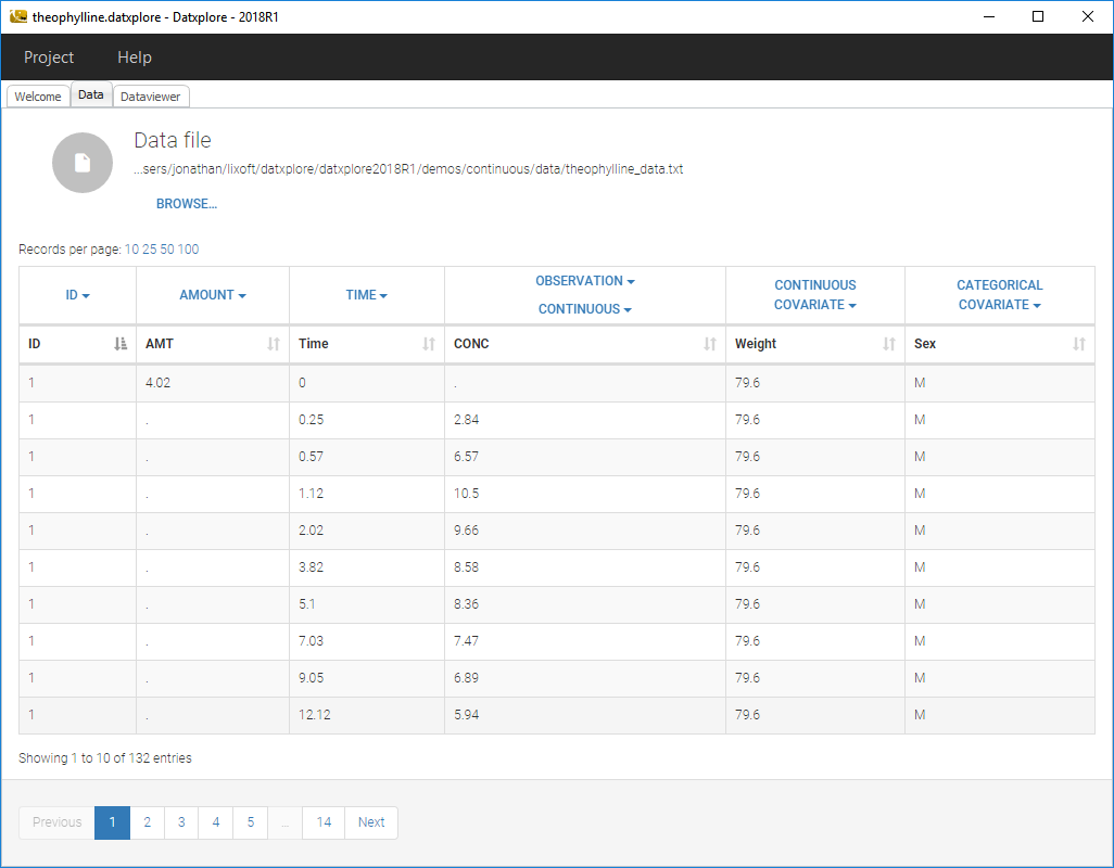
- A window with all the demos for Datxplore pops up. Then, choose the file theophylline.datxplore in the folder continuous and click on open.
- Datxplore should load the project and display the data set like on the following figure.
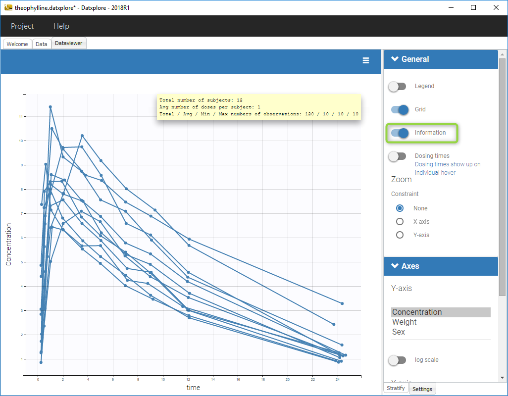
- Click on the Dataviewer frame and the following figure should appear should load the project and display the data set like on the following figure.
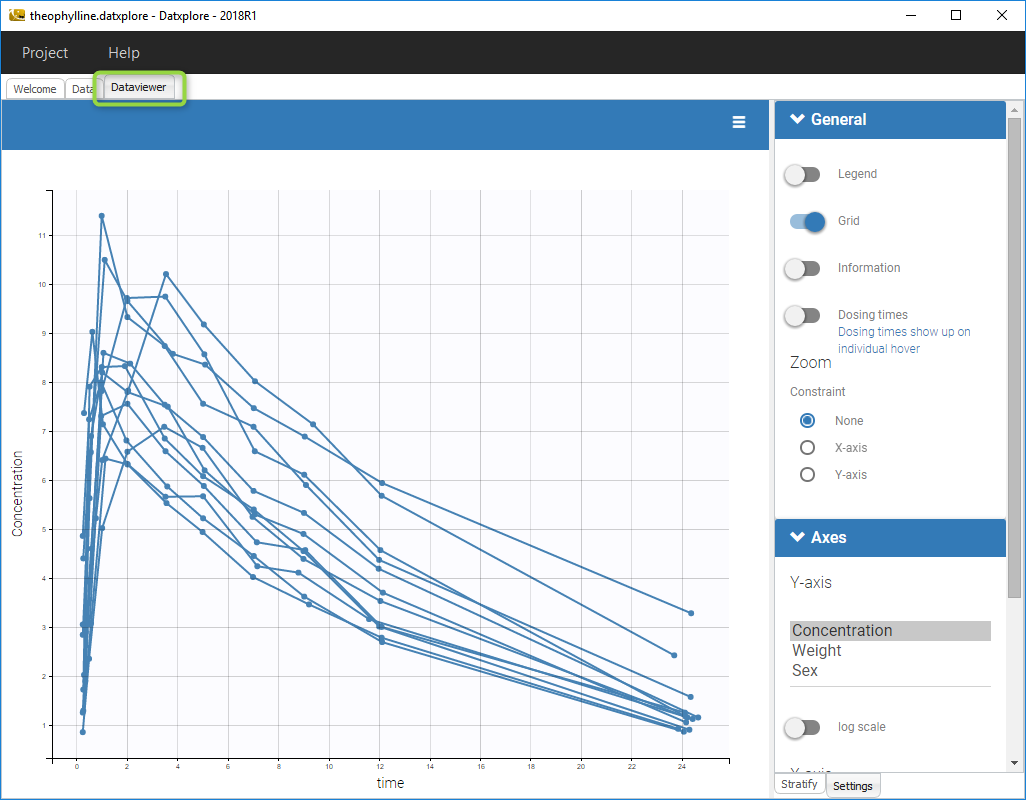
- Click on the toggle next to information to see all the informations concerning the data set
Mlxplore
- Open Mlxplore
- Go to the menu Project/Load demo as on the following figure
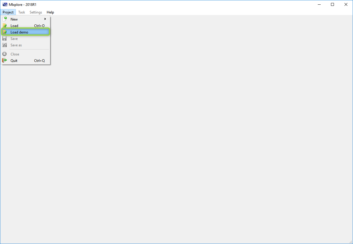
- A window with all the demos for Mlxplore pops up. Then, choose the file TumorGrowthModel.mlxplore in the folder CaseStudiesTumorGrowthInhibitionModel and click on open.
- Mlxplore loads the project and display the model like on the following figure.
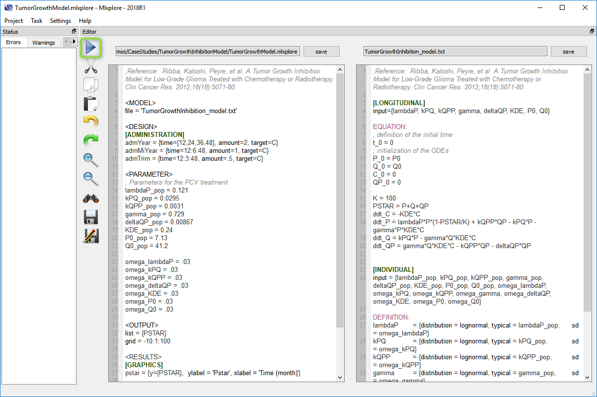
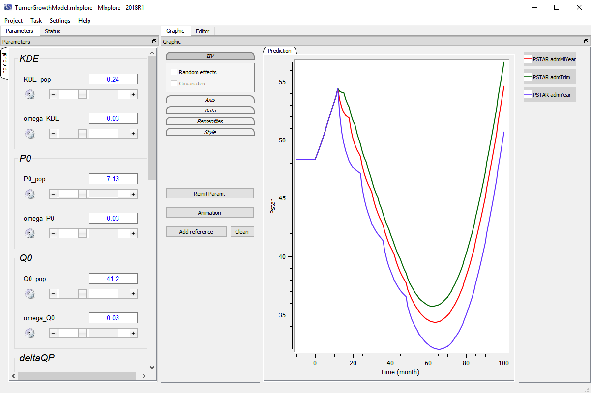
- Run the project bu clicking on the arrow (in the green circle). The computation will run and the following figure is displayed
Monolix
- Open Monolix
- Go to the menu Demos and choose theophylinne_project is section 1.1
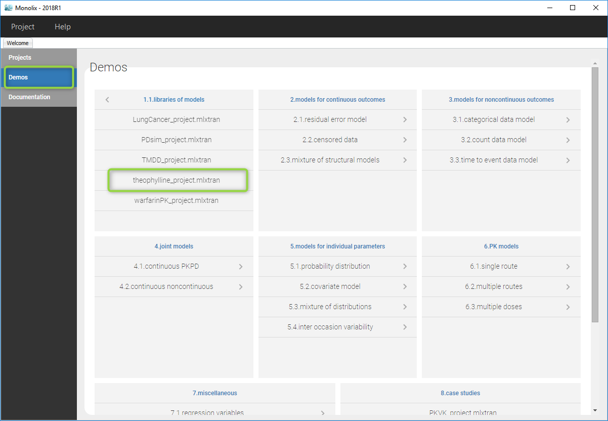
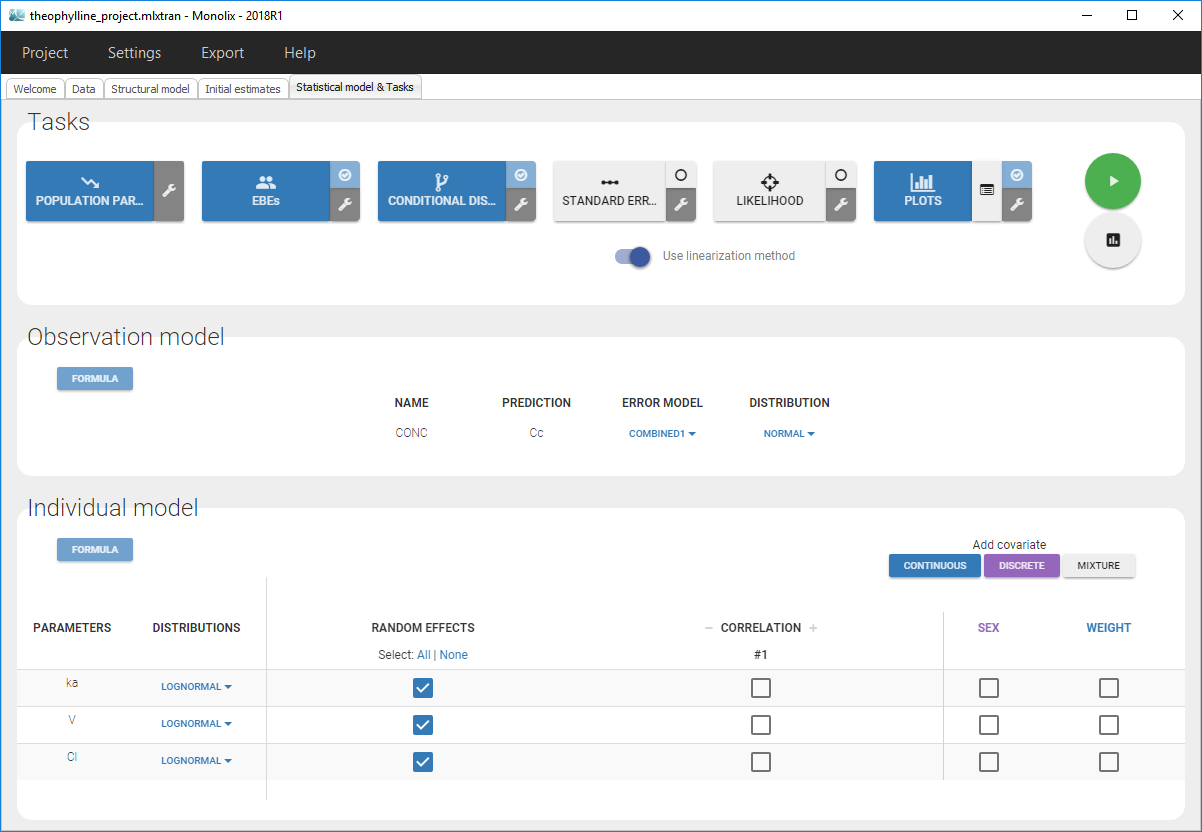
- Monolix loads the project and the interface looks like the following figure
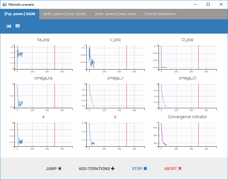
- Clicking on the “Run” button launches the scenario as on the following figure
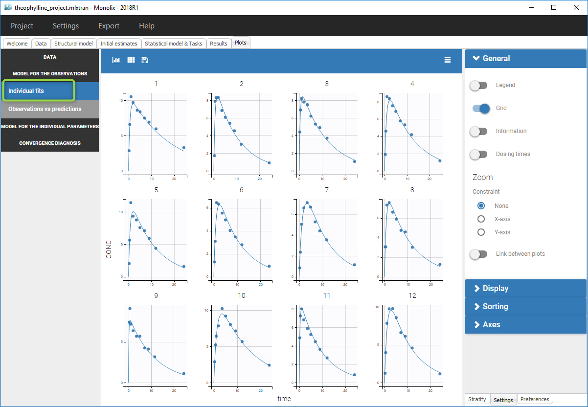
- Close the scenario using the close button and the graphics are displayed behind on the Individual fits plot
Simulx
Simulx is a little bit different from the other applications because it does not have yet a user interface. To validate it, one should use R (version greater than 3.0.2) to run simulations.
- Open R or Rstudio
- The R-packages needed to run Simulx are defined here. Make sure you have all the required packages.
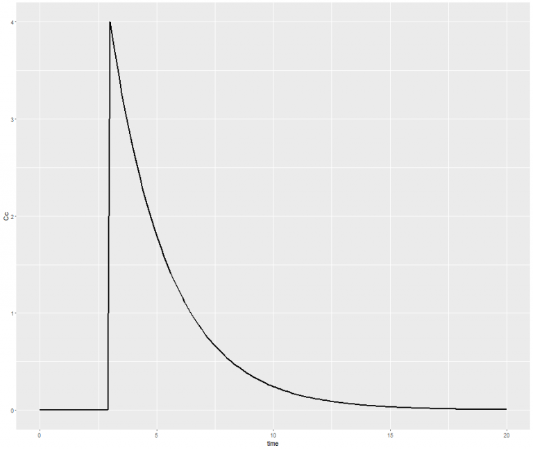
- Execute the following commands
# Define the mlxR library library("mlxR") # Define the model myModel <- inlineModel("[LONGITUDINAL] input = {V, Cl} EQUATION: Cc = pkmodel(V, Cl)") # Define the administration adm <- list(time=3, amount=40) # Define the output Cc <- list(name='Cc',time=seq(from=0, to=20, by=0.1)) # Run the simulation res <- simulx(model=myModel, parameter=c(V=10, Cl=4), output=Cc,treatment=adm) # Plot the concentration w.r.t. time print(ggplot(data=res$Cc, aes(x=time, y=Cc)) + geom_line(size=1)) - The computation is launched and the following graphic appears